Couple Cluster theory

Ground state

The CC wavefunction can be written as:

$\Psi_{\text{CC}} = e^T |\Phi_0\rangle$

The cluster operator $T$ can be expressed as:

$T = T_1 + T_2 + T_3 + \dots$

where the $T_n$ operator is defined as:

$T_n = \frac{1}{n!^2}\sum t_{ijk\dots}^{abc\dots} a^\dagger ib^\dagger jc^\dagger k\dots$

For example, the single excitation operator $T_1$ is defined as:

$T_1 = \sum_{ia} t_i^a a^\dagger i$

and the double excitation operator $T_2$ is defined as:

$T_2 = \frac{1}{4}\sum_{ijab} t_{ij}^{ab} a^\dagger ib^\dagger j$

The exponential operator $e^T$ can be expanded as:

$\begin{aligned} e^T = & 1 + T + \frac{1}{2}T^2 + \frac{1}{3!}T^3 + \dots \\ = & 1 + T_1 + T_2 + \dots \\ & + \frac{1}{2}T_1^2 + T_1T_2 + \frac{1}{2}T_2^2 + \dots \\ & + \frac{1}{3!}T_1^3 + \frac{1}{2}T_1^2T_2 + \frac{1}{2}T_1T_2^2 + \frac{1}{3!}T_2^3 + \dots \end{aligned}$

The single excitation can be expressed as:

$\Phi_1 = T_1 |\Phi_0\rangle$

and the double excitation can be expressed as:

$\Phi_2 = (T_2 + \frac{1}{2}T_1^2 )|\Phi_0\rangle$

Return to the Schrödinger equation, we can obtain that:

$\hat{H} \Psi_\text{CC} = \hat{H} e^T |\Phi_0\rangle = E e^T |\Phi_0\rangle$

Multiplying the equation by $e^{-T}$ from the left, we can obtain:

$e^{-T} \hat{H} e^T |\Phi_0\rangle = E |\Phi_0\rangle$

We introduce the effective Hamiltonian (similarity transformed Hamiltonian):

$\bar{H} = e^{-T}H e^T$

Therefore, the equation can be rewritten as:

$\bar{H} |\Phi_0\rangle = E |\Phi_0\rangle$

By projecting onto excitation determinants, we can obtain:

$\langle \Phi_{ij\dots}^{ab\dots} | \bar{H} | \Phi_0 \rangle = 0$

where $\Phi_{ij\dots}^{ab\dots}$ is the excitation determinant.

The ground state energy can be expressed as:

$E_{\text{CC}} = \langle \Phi_0 | \bar{H} | \Phi_0 \rangle$

The electronic Hamiltonian operator can be expressed as:

$\hat{H} = E_{\text{HF}} + \sum_{pq} F_{pq} p^\dagger q + \frac{1}{4} \sum_{pqrs} \langle pq||rs \rangle p^\dagger q^\dagger s r$

There are four terms in the one electron operator: OO, OV, VO, and VV. For the two-electron operator, there are 9 distinct terms: OOOO, OOOV, OVOO, OOVV, VVOO, OVOV, VOVV, VVVO, VVVV.

The effective Hamiltonian can be rewritten using Baker-Campbell-Hausdorff formula as:

$\begin{aligned} \bar{H} = & \hat{H} + \left[\hat{H}, T\right] + \frac{1}{2!}\left[\left[\hat{H}, T\right], T\right] + \dots \\ = & \hat{H} + \left[\hat{H}, T_1\right] + \left[\hat{H}, T_2\right] + \frac{1}{2}\left[\left[\hat{H}, T_1\right], T_1\right] \\ & + \frac{1}{2}\left[\left[\hat{H}, T_2\right], T_2\right] + \left[\left[\hat{H}, T_1\right], T_2\right] + \dots \end{aligned}$

knowing that:

$\begin{aligned} \left[\left[\hat{H}, T_1\right], T_2\right] = \left[\left[\hat{H}, T_2\right], T_1\right] \end{aligned}$

Only the single and double cluster amplitudes contribute to the CC energy (that means only consider the contribution of single and double), and therefore the energy can be expressed as:

$\begin{aligned} E_{\text{CC}} & = \langle \Phi_0 | \bar{H} |\Phi_0 \rangle \\ & = \langle \Phi_0 | \hat{H} | \Phi_0 \rangle + \sum_{ia} F_{ia} t_i^a + \frac{1}{2} \sum_{ijab} \langle ij||ab \rangle t_{i}^{a} t_{j}^{b} + \frac{1}{4} \sum_{ijab} \langle ij||ab \rangle t_{ij}^{ab} \\ & = E_{\text{HF}} + \sum_{ia} F_{ia} t_i^a + \frac{1}{4} \sum_{ijab} \langle ij||ab \rangle(t_{ij}^{ab}+t_{i}^{a} t_{j}^{b} -t_{i}^{b} t_{j}^{a} ) \end{aligned}$

where $F_{ia}$ is the Fock matrix element, and $\langle ij||ab \rangle$ is the two-electron integral. The $\langle \Phi_0 | \hat{H} | \Phi_0 \rangle$ equals to the Hartree-Fock energy $E_{\text{HF}}$ .

CCSD

In CCSD, the cluster operator is truncated at the single and double excitation level:

$T = T_1 + T_2$

and the wavefunction can be expressed as:

$|\Psi_{\text{CCSD}} \rangle = e^{T_1+T_2} |\Phi_0\rangle$

Projecting onto singly and doubly excited determinants, we can obtain:

$\langle \Phi_{i}^{a} | e^{-T_1}\hat{H}e^{T_1} + \left[e^{-T_1}\hat{H}e^{T_1}, T_2\right] | \Phi_0 \rangle = 0$

$\begin{aligned} & \langle \Phi_{ij}^{ab} | e^{-T_2-T_1}\hat{H}e^{T_1+T_2} | \Phi_0 \rangle = \langle \Phi_{ij}^{ab} | e^{-T_2}e^{-T_1}\hat{H}e^{T_1}e^{T_2} | \Phi_0 \rangle \\ & = \langle \Phi_{ij}^{ab} | e^{-T_1}\hat{H}e^{T_1} + \left[e^{-T_1}\hat{H}e^{T_1}, T_2\right] + \frac{1}{2}\left[\left[e^{-T_1}\hat{H}e^{T_1}, T_2\right], T_2\right] | \Phi_0 \rangle = 0 \end{aligned}$

The energy can be expressed as:

$E_{\text{CCSD}} = \sum_a\sum_i t_i^a f_{ia} + \frac{1}{4} \sum_{ab}\sum_{ij}\tau_{ij}^{ab} \langle ij||ab \rangle$

CC2

In the CC2 method, the projection onto the singly excited determinant is the same as the CCSD method:

$\langle \Phi_{i}^{a} | e^{-T_1}\hat{H}e^{T_1} + \left[e^{-T_1}\hat{H}e^{T_1}, T_2\right] | \Phi_0 \rangle = 0$

and the projection onto the doubly excited determinant is:

$\langle \Phi_{ij}^{ab} | e^{-T_1}\hat{H}e^{T_1} + \left[F, T_2\right] | \Phi_0 \rangle = 0$

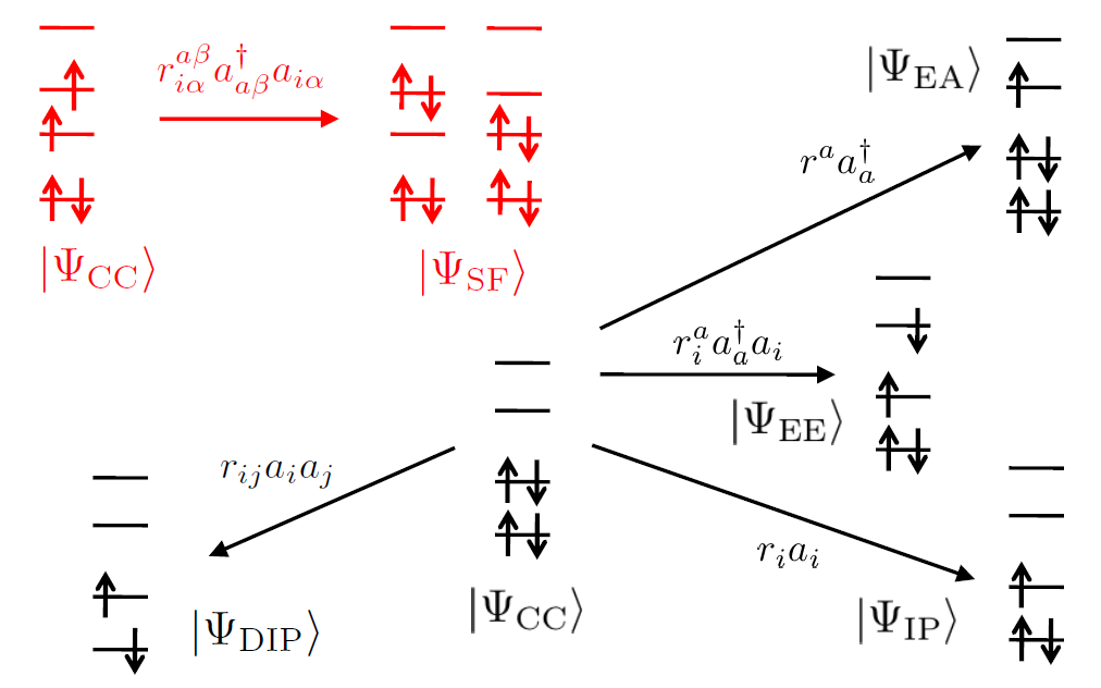
EOM-CC

EOM-EE (Electronically Excited States)

Excited state can be expressed as:

$|\Psi_{\text{ex}}\rangle = \mathbf{R} |\Phi_\text{g}\rangle$

where $|\Psi_{\text{ex}}\rangle$ is the excited state, and $|\Phi_\text{g}\rangle$ is the ground state. $\mathbf{R}$ is the excitation operator, which can be expressed as:

$\mathbf{R} = \sum_{n} \mathbf{R}_n$

$\mathbf{R}_n = \frac{1}{n!^2}\sum r_{ijk\dots}^{abc\dots} a^\dagger ib^\dagger jc^\dagger k\dots$

The ground state is approximated by:

$|\Phi_\text{g}\rangle = e^T |\Phi_0\rangle$

where $|\Phi_0\rangle$ is an arbitrary Slater determinant, usually SCF solution.

Therefore, the excited state can be expressed as:

$|\Psi_{\text{ex}}\rangle =\mathbf{R} e^T |\Phi_0\rangle = e^T \mathbf{R} |\Phi_0\rangle$

which means the right excitation operator $\mathbf{R}$ and the cluster operator $T$ are commutative.

Inserting the equation into the Schrödinger equation, we can obtain:

$H \mathbf{R} e^T |\Phi_0\rangle = E_\text{ex} \mathbf{R} e^T |\Phi_0\rangle$

The $T$ operator and $\mathbf{R}$ operator are necessarily commutative, so we can rewrite the equation using the effective Hamiltonian operator $\bar{H}= e^{-T}H e^T$ :

$e^{-T}H e^T \mathbf{R} |\Phi_0\rangle = \bar{H} \mathbf{R} |\Phi_0\rangle = E_\text{ex} \mathbf{R} |\Phi_0\rangle$

and then we can obtain the equation:

$(\bar{H}-E_\text{ex}) \mathbf{R} |\Phi_0\rangle = 0$

The goal of any EOM-CC calculation is to determine the energy difference between the initial and target states:

$\omega_k = E_k - E_{\text{CC}}$

With the commutation relation between the cluster operator $T$ and the excitation operator $\mathbf{R}$ , we can obtain the EOM-CC equation:

$[\bar{H},\mathbf{R}]|\Phi_0\rangle = \omega_k \mathbf{R}|\Phi_0\rangle$

The effective Hamiltonian can be expressed in spin-orbital basis as:

$\bar{H} = \sum_{pq} \mathbf{F}_{pq} a^\dagger_p a_q + \frac{1}{4} \sum_{pqrs} \mathbf{W}_{pqsr} a^\dagger_p a^\dagger_q a_s a_r$

Note that the CC wave operator $e^T$ is not unitary, so the effective Hamiltonian $\bar{H}$ is not Hermitian. As a result, each root of $\bar{H}$ is associated with two eigenvectors, which are the left and right eigenvectors. The left eigenvector is defined as:

$\langle \tilde{\Psi} | = \langle \Psi_L | = \langle \Phi_0 | \mathbf{L} e^{-T}$

and the right eigenvector is defined as:

$| \Psi \rangle = | \Psi_R \rangle = e^T \mathbf{R} |\Phi_0 \rangle$

Note that the left deexcitation operator $\mathbf{L}$ is not commutative with the cluster operator $T$ . The left eigenfunction is defined as:

$\langle \Psi_0 | \mathbf{L}\bar{H} = \langle \Phi_0 | \mathbf{L}\omega_k$

The left de-excitation operator $\mathbf{L}$ can be expressed as:

$\mathbf{L} = \sum_{n} \mathbf{L}_n$

$\mathbf{L}_n = \frac{1}{n!^2}\sum l_{abc\dots}^{ijk\dots} i^\dagger aj^\dagger bk^\dagger c\dots$

The left and right operators satisfy the biorthogonality condition:

$\langle \mathbf{L}_i | \mathbf{R}_j \rangle = \delta_{ij}$

The two sets of solutions satisfy the biorthogonality condition:

$\langle \tilde{\Psi}^{(i)} | \Psi^{(j)} \rangle = 1$

If the C is unity, we can rewrite the equation as:

$\langle \tilde{\Psi} | \Psi \rangle = 1$

and therefore the energy can be expressed as:

$E = \langle \tilde{\Psi} | H | \Psi \rangle = \langle \Phi_0 |\mathbf{L} \bar{H} \mathbf{R}| \Phi_0 \rangle$

Note that for ground state, we have $\mathbf{L} = \mathbf{R} = 1$ , so the energy can be expressed as:

$E_{\text{CC}} = \langle \Phi_0 | \bar{H} | \Phi_0 \rangle$

The eigenvalues can be obtained by diagonalizing the matrix $\mathbf{A}$ in the basis of the reference, single excited and doubly excited determinants. The Jacobian matrix can be expressed as:

$\mathbf{A} = \begin{pmatrix} \langle\Phi_i^a|[\tilde{H}+[\tilde{H},T_2],\{c^\dagger k\} ]| \Phi_0\rangle & \langle\Phi_i^a|[\tilde{H},\{c^\dagger d^\dagger kl\} ]| \Phi_0\rangle \\ \langle\Phi_{ij}^{ab}|[\tilde{H}+[\tilde{H},T_2],\{c^\dagger k\}] | \Phi_0\rangle & \langle\Phi_{ij}^{ab}|\tilde{H}+[\tilde{H},T_2],\{c^\dagger d^\dagger kl\} | \Phi_0\rangle \end{pmatrix}$

For CC2, the Jacobian matrix can be expressed as:

$\mathbf{A} = \begin{pmatrix} \langle\Phi_i^a|[\tilde{H}+[\tilde{H},T_2],\{c^\dagger k\} ]| \Phi_0\rangle & \langle\Phi_i^a|[\tilde{H},\{c^\dagger d^\dagger kl\} ]| \Phi_0\rangle \\ \langle\Phi_{ij}^{ab}|[\tilde{H},\{c^\dagger k\}] | \Phi_0\rangle & \langle\Phi_{ij}^{ab}|F,\{c^\dagger d^\dagger kl\} | \Phi_0\rangle \end{pmatrix}$

And the whole eigenfunction can be expressed as:

$\mathbf{A} \begin{pmatrix} R_1 \\ R_2 \end{pmatrix} = \omega \begin{pmatrix} R_1 \\ R_2 \end{pmatrix}$

$\begin{pmatrix} L_1 & L_2 \end{pmatrix} \mathbf{A} = \begin{pmatrix} L_1 & L_2 \end{pmatrix}\omega$

Then, the right and left eigenfunctions can be expressed as:

$\sum_{kc}\langle\Phi_i^a|[\tilde{H}+[\tilde{H},T_2],\{c^\dagger k\} ]| \Phi_0\rangle r_k^c + \sum_{klcd} \langle\Phi_i^a|[\tilde{H},\{c^\dagger d^\dagger kl\} ]| \Phi_0\rangle r_{kl}^{cd} = \omega r_i^a$

$\sum_{kc}\langle\Phi_{ij}^{ab}|[\tilde{H}+[\tilde{H},T_2],\{c^\dagger k\}] | \Phi_0\rangle r_k^c + \sum_{klcd} \langle\Phi_{ij}^{ab}|\tilde{H}+[\tilde{H},T_2],\{c^\dagger d^\dagger kl\} | \Phi_0\rangle = \omega r_{ij}^{ab}$

$\sum_{ia}l_a^i \langle\Phi_i^a|[\tilde{H}+[\tilde{H},T_2],\{c^\dagger k\} ]| \Phi_0\rangle + \sum_{ijab} l_{ij}^{ab} \langle\Phi_{ij}^{ab}|[\tilde{H}+[\tilde{H},T_2],\{c^\dagger k\}] | \Phi_0\rangle = \omega l_k^c$

$\sum_{ia}l_a^i\langle\Phi_i^a|[\tilde{H},\{c^\dagger d^\dagger kl\} ]| \Phi_0\rangle + \sum_{ijab} l_{ij}^{ab} \langle\Phi_{ij}^{ab}|\tilde{H}+[\tilde{H},T_2],\{c^\dagger d^\dagger kl\} | \Phi_0\rangle = \omega l_{kl}^{cd}$

EOM-EA (Electron Attachment)

For EOM-EA state, the right excitation operator $\mathbf{R}$ is defined as:

$\mathbf{R}^{\text{EA}} = \sum_{a} r_a a^\dagger + \frac{1}{2} \sum_{iab} r_{i}^{ab} ia^\dagger b^\dagger + \cdots$

EOM-IP (Ionization Potential)

For EOM-IP state, the right excitation operator $\mathbf{R}$ is defined as:

$\mathbf{R}^{\text{IP}} = \sum_{i} r_i i + \frac{1}{2} \sum_{ija} r_{ij}^{a} ija^\dagger + \cdots$

EOM-SF (Spin-Flip)

For EOM-SF state, the right excitation operator $\mathbf{R}$ is defined as:

$\mathbf{R}_{M_s=-1} \equiv \mathbf{R}^{\text{IP}} = \sum_{ia}r_i^aa_\beta^\dagger i_\alpha + \frac{1}{2}\sum_{ijab}r_{ij}^{ab}a_\beta^\dagger i_\alpha b_\sigma^\dagger j_\sigma + \cdots$

where $\sigma=\alpha$ or $\beta$ .

Derivative

General

The asymmetrized, perturbation-independent, deexcitation operator $\Lambda$ can be expressed as:

$\begin{aligned} & \Lambda = \sum_{n} \Lambda_n \\ & \Lambda_1 = \sum_{ia} \lambda_i^a i^\dagger a \\ & \Lambda_2 = \frac{1}{4}\sum_{ijab} \lambda_{ij}^{ab} a_i^\dagger a_j^\dagger a_b a_a \\ & \Lambda_n = \frac{1}{n!^2}\sum \lambda_{abc\dots}^{ijk\dots} i^\dagger aj^\dagger bk^\dagger c\dots \end{aligned}$

The $\lambda$ amplitude satisfies the condition:

$\langle \Phi_0 | \Lambda | \Phi \rangle = - \langle \Phi_0 | (H_Ne^T)_c | \Phi \rangle \langle \Phi | (H_Ne^T)_c - \Delta E| \Phi \rangle ^{-1}$

Therefore, we have:

Finally the derivative of the energy can be expressed as:

$\begin{aligned} \Delta E^\xi = & \mathbf{D}_{ij}f_{ij}^\xi + \mathbf{D}_{ab}f_{ab}^\xi + \sum_{pqrs}\Gamma(pq,rs) \langle pq||rs \rangle^\xi \\ = & \mathbf{D}_{ij}f_{ij}^\xi + \mathbf{D}_{ab}f_{ab}^\xi \\ & + \Gamma(ij,ab)\langle ij||ab\rangle^\xi + \Gamma(ab,cd)\langle ab||cd\rangle^\xi \\ & + \Gamma(kl,ij)\langle kl||ij\rangle^\xi + \Gamma(ja,bi)\langle ja||bi\rangle^\xi \\ & + \Gamma(ai,bc)\langle ai||bc\rangle^\xi + \Gamma(jk,ia)\langle jk||ia\rangle^\xi \\ \end{aligned}$

where the $D_{pq}$ is the relaxed density matrix, and the $\Gamma_{pq,rs}$ is the effective density matrix.

CCSD Derivative

The CCSD gradient can be expressed as:

$\frac{\partial E_{\text{CCSD}}}{\partial \xi} = \sum_{pq} D_{pq}f_{pq}^{(\xi)} + \sum_{pqrs}\Gamma(pq,rs) \langle pq||rs \rangle^\xi + \sum_{pq}I_{pq}S_{pq}^{\xi}$

EOM-CC Derivative

The derivative of the EOM-CC energy can be expressed as:

$\frac{\partial E_{\text{EOM-CC}}}{\partial \xi} = D_{pq}f_{pq}^{(\xi)} + \frac{1}{4}\Gamma_{pqrs} \langle pq||rs \rangle^\xi + I_{pq}S_{pq}^{\xi}$

where: overlap derivative:

$S_{pq}^{\xi} = c_{\mu p} \frac{\partial S_{\mu\nu}}{\partial \xi} c_{\nu q} = c_{\mu p} c_{\nu q} \left( \langle \frac{\partial\chi_\mu}{\partial\xi}|\chi_\nu \rangle + \langle \chi_\mu|\frac{\partial\chi_\nu}{\partial\xi} \rangle \right)$

ERI derivative:

$\langle pq||rs \rangle^\xi = c_{\mu p} c_{\nu q} c_{\lambda r} c_{\sigma s} \frac{\partial \langle \mu\lambda||\nu\sigma \rangle}{\partial \xi}$

$\phi_p = c_{\mu p} \xi_{\mu}$

Fock matrix derivative:

$f_{pq}^{(\xi)} = c_{\mu p}c_{\nu q} \left(\frac{\partial h_{\mu\nu}}{\partial\xi}+ c_{\lambda i}c_{\sigma i}\frac{\partial\langle \mu\lambda||\nu\sigma \rangle}{\partial\xi} \right) = h_{pq}^\xi + \sum_{m} \langle pm||qm \rangle^\xi$

Derivative of the MO coefficients:

$\frac{\partial c_{\mu p}}{\partial \xi} = \sum_q U_{qp}^\xi c_{\mu q}$

where $U_{qp}^\xi$ is the CPHF coefficient.

Relaxed density matrix:

$D_{pq} = \gamma_{pq} + z_{pq}$

Effective density matrix:

$\gamma_{pq} = \langle \Phi_0 | \mathbf{L}[p^\dagger qe^T]_c\mathbf{R} |\Phi_0 \rangle + \langle \Phi_0 | \mathcal{Z}[p^\dagger qe^T]_c|\Phi_0 \rangle$

$\Gamma_{pqrs} = \langle \Phi_0 | \mathbf{L}[p^\dagger q^\dagger sr e^T]_c\mathbf{R} |\Phi_0 \rangle + \langle \Phi_0 | \mathcal{Z}[p^\dagger q^\dagger sr e^T]_c|\Phi_0 \rangle$

where $c$ indicates the limitation to connected diagrams.

Auxiliary deexcitation operator $\mathcal{Z}$ :

$\mathcal{Z} = \sum_{n} \mathcal{Z}_n$

$\mathcal{Z}_n = \frac{1}{n!^2}\sum \zeta_{abc\dots}^{ijk\dots} i^\dagger aj^\dagger bk^\dagger c\dots$

Lagrangian of EOM-CC derivative

The EOM energy can be expressed as:

The full energy derivative can be expressed as:

$\frac{\mathrm{d} E }{\mathrm{d} \xi} = \frac{\partial E}{\partial \xi} + \frac{\partial E}{\partial L}\frac{\partial L}{\partial \xi} + \frac{\partial E}{\partial R}\frac{\partial R}{\partial \xi} + \frac{\partial E}{\partial T}\frac{\partial T}{\partial \xi} + \frac{\partial E}{\partial C}\frac{\partial C}{\partial \xi}$

The first term is the Hellmann-Feynman contribution:

$\begin{aligned} & \frac{\partial E}{\partial \xi} = \sum_{pq} h_{pq}^\xi \gamma_{pq}' + \frac{1}{4}\sum_{pqrs}\langle pq||rs \rangle^\xi \Gamma_{pqrs}' \\ & h_{pq}^\xi = \frac{\partial h_{pq}}{\partial \xi} = \sum_{\mu\nu}C_{\mu p}h_{\mu\nu}^\xi C_{\nu q} \\ & h_{\mu\nu}^\xi = \langle \chi_\mu | \frac{\partial \hat{h}}{\partial \xi} | \chi_\nu \rangle + \langle \frac{\partial \chi_\mu}{\partial\xi} | \hat{h} | \chi_\nu \rangle + \langle \chi_\mu | \hat{h} | \frac{\partial \chi_\nu}{\partial\xi} \rangle \\ & \langle pq||rs \rangle^\xi = \frac{\partial \langle pq||rs \rangle}{\partial \xi} = \sum_{\mu\nu\lambda\sigma}C_{\mu p}C_{\nu q}\langle \chi_\mu\chi_\nu||\chi_\lambda\chi_\sigma \rangle^\xi C_{\lambda r}C_{\sigma s} \\ \end{aligned}$

$\begin{aligned} \langle \chi_\mu\chi_\nu||\chi_\lambda\chi_\sigma \rangle^\xi = & \langle \frac{\partial \chi_\mu}{\partial\xi}\chi_\nu||\chi_\lambda\chi_\sigma \rangle + \langle \chi_\mu\frac{\partial \chi_\nu}{\partial\xi}||\chi_\lambda\chi_\sigma \rangle \\ & + \langle \chi_\mu\chi_\nu||\frac{\partial \chi_\lambda}{\partial\xi}\chi_\sigma \rangle + \langle \chi_\mu\chi_\nu||\chi_\lambda\frac{\partial \chi_\sigma}{\partial\xi} \rangle \end{aligned}$

The EOM energy is stationary with respect to the left and right eigenvectors, so the second and third terms are zero:

$\frac{\partial E}{\partial L} = \frac{\partial E}{\partial R} = 0$

Then there is so-called amplitude response $\frac{\partial E}{\partial T}$ and orbital response $\frac{\partial E}{\partial C}$ .

The Lagrangian derivative can be expressed as:

$\begin{aligned} \frac{\partial \mathcal{L}(L, R, T, C,Z, \Lambda, \Omega)}{\partial \xi} = & \langle \Phi_0 Le^{-T} | \frac{\partial H}{\partial\xi} | e^TR\Phi_0 \rangle \\ + & \langle \Phi_0 Ze^{-T} | \frac{\partial H}{\partial\xi} | e^T\Phi_0 \rangle \\ + & \frac{1}{2}\sum_{pq}\lambda_{pq}\frac{\partial f_{pq}}{\partial\xi} + \sum_{pq}\omega_{pq}\frac{\partial S_{pq}}{\partial\xi} \\ = & \sum_{pq}h_{pq}^\xi\rho_{pq} + \frac{1}{4}\sum_{pqrs}\langle pq||rs \rangle^\xi \Pi_{pqrs} \\ + & \sum_{pq}\omega_{pq}S_{pq}^{\xi} \end{aligned}$

The effective density matrices $\rho$ and $\Pi$ can be expressed as:

$\begin{aligned} & \rho = \gamma' + \gamma'' + \gamma''' \\ & \Pi = \Gamma' + \Gamma'' + \Gamma''' \end{aligned}$

where the $\gamma'$ and $\Gamma'$ are the so-called non-relaxed density matrices:

$\begin{aligned} & \gamma' = \frac{1}{2}\langle \Psi_L | p^\dagger q+q^\dagger p |\Psi_R \rangle \\ & \Gamma' = \frac{1}{2}\langle \Psi_L | p^\dagger q^\dagger sr + s^\dagger r^\dagger pq |\Psi_R \rangle \end{aligned}$

and $\gamma''$ and $\Gamma''$ are amplitude response contributions:

$\begin{aligned} & \gamma'' = \frac{1}{2}\langle \Phi_0Ze^{-T} | p^\dagger q+q^\dagger p |e^T\Phi_0 \rangle \\ & \Gamma'' = \frac{1}{2}\langle \Phi_0Ze^{-T} | p^\dagger q^\dagger sr + s^\dagger r^\dagger pq |e^T\Phi_0 \rangle \end{aligned}$

and $\gamma'''$ and $\Gamma'''$ are orbital response contributions. $\gamma'''$ is related to the Lagrange multiplier $\lambda$ , and $\Gamma'''$ is related to $\gamma'''$ and $\delta$ .

Properties

Different CC2 variants: